JUNE 2022 - SIMULATIONS
The final newsletter on spatial variability discusses methods for simulating it. If one knows the trend, amount and speed of variation, potential situations can be simulated. This can benefit designs (by foreseeing the unforeseen) and operations (by predicting likely upcoming situations). It took a while to publish a new update due to a busy period and a month of holiday! Hopefully that improves a bit!
TOPIC OF TODAY #1 - INGREDIENTS OF A SIMULATION
It is important that all input data is correct and complete before starting with simulating the data. In the case of our soil data (CPT measurements) this requires clustering (see this edition) and determining the following variability descriptors (see this edition):
- Trendline around which the fluctuation will occur (can be any trendline, does not have to be linear)
- Distribution type and parameters of the variation which determine the size and likelihood of certain variations
- Scale of flutuation which determines how fast the variation along the trendline occurs
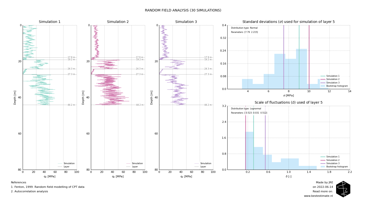
The beauty of these ingredients is that they together allow for all kind of different likely soil profiles to be simulated. These range from very likely to less likely but are all to be accounted for in the design or operation. This makes sure that your design and/or operation is robust and at the same time not overconservative. The Figure below shows the first 3 of (in total 30) simulations.

TOPIC OF TODAY #2 - IMPACT OF PARAMETER SIMULATIONS
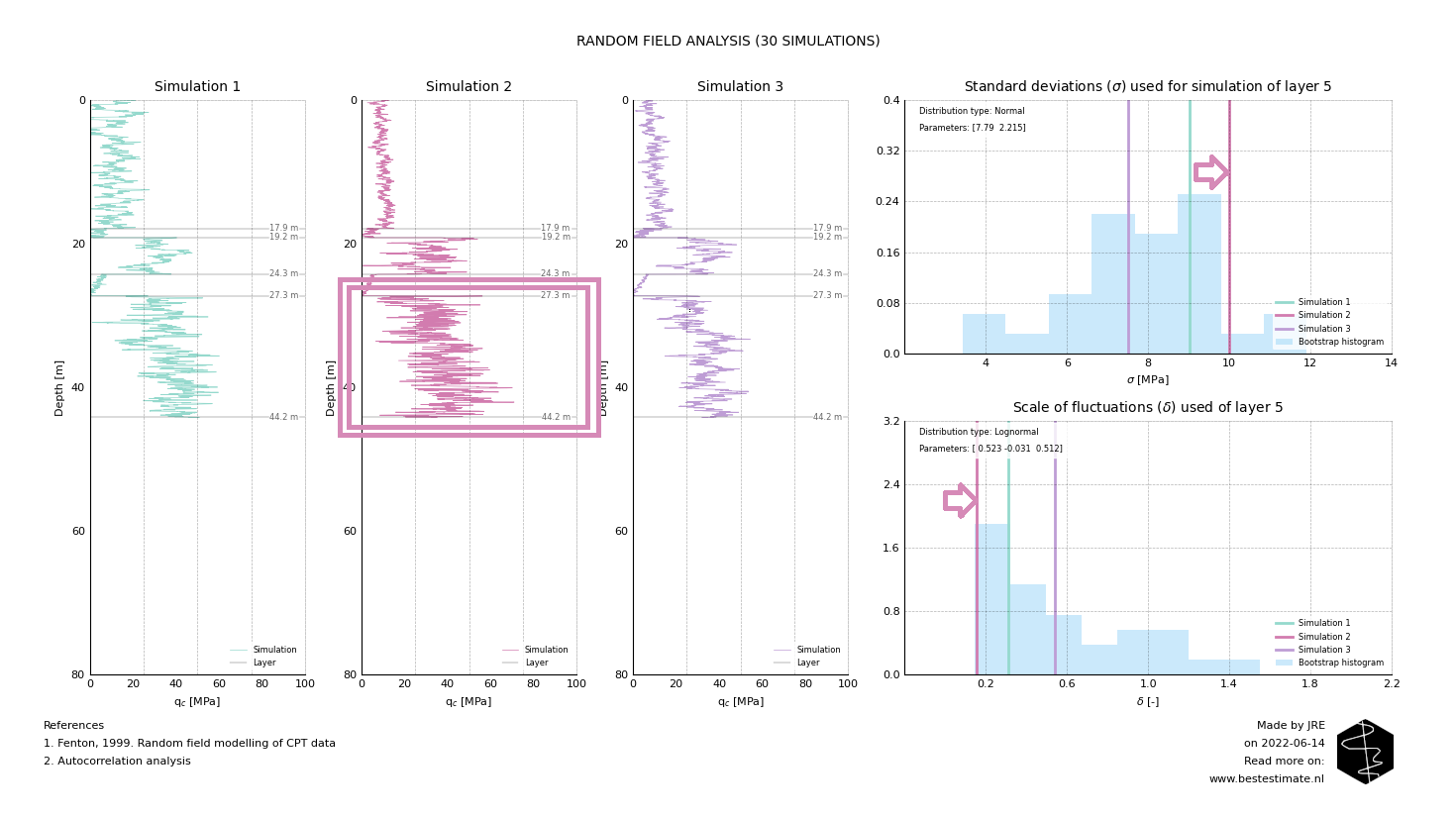
The variation of the standard deviation and scale of fluctuation is often ignored but is very important. The input data for the 5th layer is displayed in both histograms on the right side. They are displayed to help out interpreting what the impact of parameter selection is. Below Figure shows the results of layer 5 in the 2nd simulated profile. As visible, the profile varies significantly faster than simulation 1 and 3. Additionally the highest and lowest values are further apart. This is the case since the scale of fluctuation is low (meaning there is little correlation over depth) and the standard deviation is high (implying a large variability).

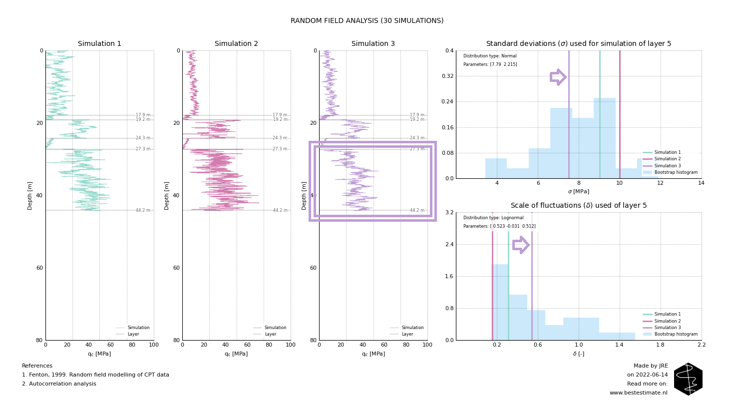
The opposite of simulation 2 happens in layer 5 of simulation 3. The scale of fluctuation is high, thus speed of variation is low. Additionally the smaller standard deviation causes less excessive variations. It is required to also include simulations like these to provide realistic input for the design. This is because the original input data shows similar variations which are properly incorporated now.

RECOMMENDATIONS FOR FURTHER DEVELOPMENT
There are many easy improvements possible to this algorithm which can make it more powerfull. Correlations between the scale of fluctuation and standard deviation can be implemented to improve accuracy of simulations (see this edition for copulas). Also variations in trendlines as well as layer depth can be incorporated. The more input data is available the more powerfull tools can be applied reliably.
Additionally using these analysis in combination with others is extra powerfull. Clustering and distribution fitting analyses can serve to create reliable input. Random field simulations can be used as input for quantile regression to create geotechnical design profiles. This is all possible given the API-based implementation. It splits all the sub-steps into small executable calculations which can interact with eachother depending on the project needs and preferences.
FOOTNOTE
Please note that I run this service besides my job at TWD. It is my ambition to continuously improve this project and publish corresponding newsletters on new innovations. In busy times this might be less, in quiet times this might be more. Any ideas? Let me know!
