JANUARY 2022 - AUTOCORRELATION
In the second newsletter on spatial variability we define two concepts used for further works. Before starting the layer identification algorithm for soils is significantly improved. Afterwards, the scale of fluctuation and autocorrelation are explained and a case study is presented.
TOPIC OF TODAY #1 - EXTRACTING A SINGLE DATA SERIES
If you properly want to assess variability of a property over time or space it is required to assure that you are evaluating one independent series. When two data series are mixed a descriptor will provide a troubled view since these data series properties differ with respect to each other. This might sound difficult in these terms, but becomes obviously clear when you read the following three examples:
- Sand and clay are present at one location at different depths. However, their data belongs to different distributions.
- Waves over time change due to a change in wind direction. Therefore the series before and after the change in weather conditions differ.
- Vessel motions in a river and on sea are siginficantly different and therefore two different series need to be assessed.
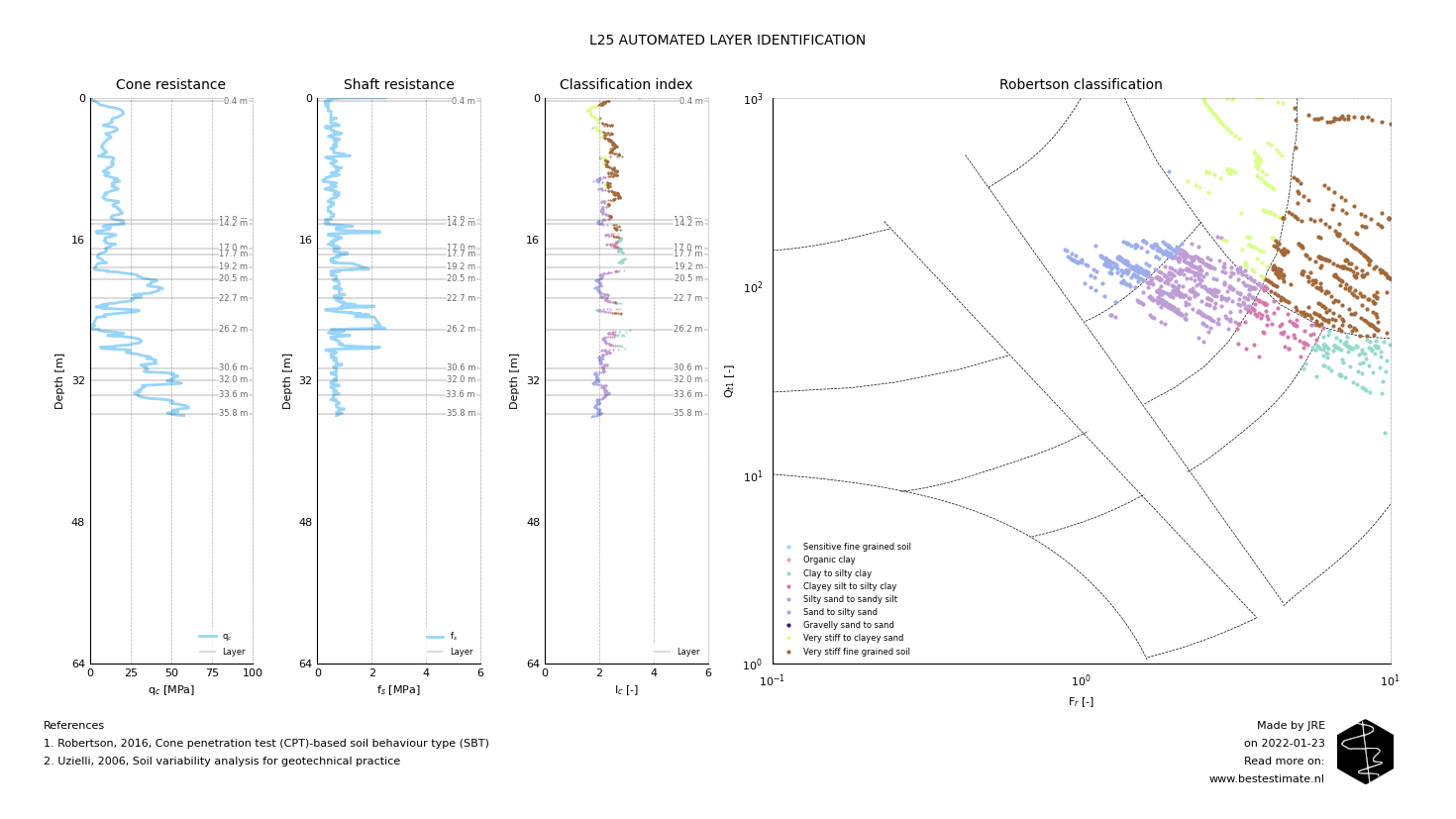
In this example soil properties over depth are evaluated. It is therefore required that different data series are constructed for each different layer. In order to do this the layer identification algorithm has been improved. This has been done by automatic merging layers based on a Welch-t tests performed between them. The figure below shows an example of the performance of this updated algorithm. As always it is possible to manually adapt the layers since engineering judgement should never be eliminated from these kind of analyses.

TOPIC OF TODAY #2 - AUTOCORRELATION
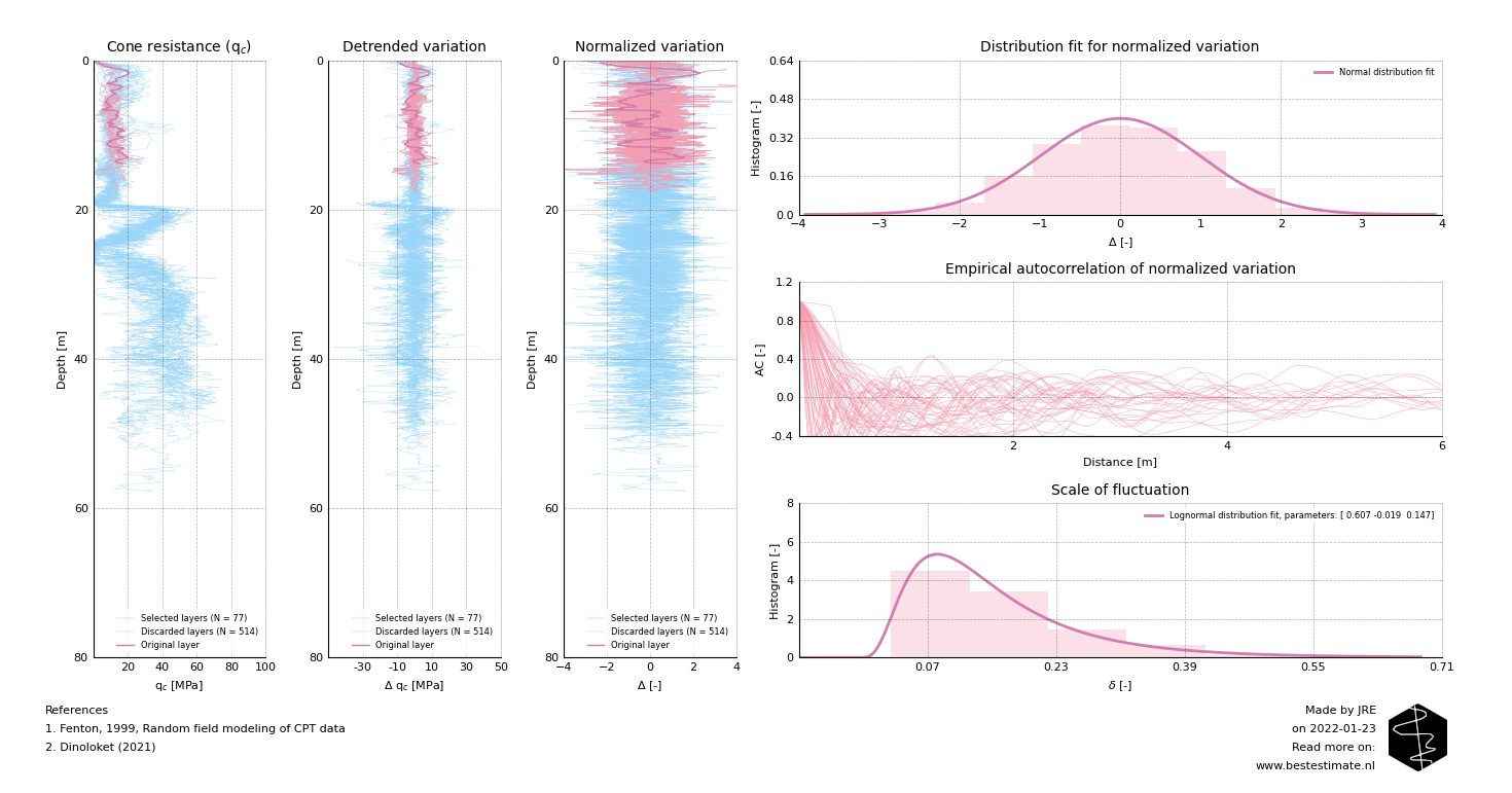
Autocorrelation is a statistical concept which describes the variation speed of a data series. This can be calculated empirically (from the actual dataset). But it is also possible to fit a theoretical function through this empirical result. That will be easier to use in further calculations. This theoretical function is often only dependent on one parameter: the scale of fluctuation (delta). The higher the scale of fluctuation, the slower the variation of the data in the series. For any data series it is most easily determined by means of the following steps:
- Identify and isolate data series (in this case soil data for one layer)
- Remove a potential trend from the data series (in this case the trendline of the cone resistance)
- Check if the distribution of the data is normal (if not theoretical autocorrelation models cannot be used)
- Normalize the data series by means of dividing by the standard deviation
- Fit a theoretical autocorrelation function and determine scale of fluctuation

As visible in the figure above it is possible to use neighbouring measurements of the same soil layer to better determine the variability of scale of fluctuation. In the case presented the scale of fluctuation can differ between 0.05 and 0.40 for the same soil type. This is because there is a variation between the measurements in the same soil types as well. In later editions an attempt will be made to use this information to try and make estimations of the potential variations of soil properties at certain locations. Other than that it is just as easily applied on vessel motions or other data as wind speed, wave height and vibrations. This allows to make safer and more economical designs.
FOOTNOTE
Please note that I run this service besides my job at TWD. It is my ambition to continuously improve this project and publish corresponding newsletters on new innovations. In busy times this might be less, in quiet times this might be more. Any ideas? Let me know!
