JUNE 2021 - COPULAS
This newsletter is a further elaboration on joint variability with a specific focus on copulas. They are from now on implemented as a possible analysis in the API. Furthermore, a case study in this newsletter shows why they are usefull. If you are not familiar with the importance of joint variabililty it is advised to read the newsletter from May 2021 first.
TOPIC OF TODAY
An offshore operation is performed in a location with waves and currents. An estimate needs to be made of the ultimate loads during the operation. The speed of the current and height of the waves determine whether the operation can be performed. The simplest and most often used method in design is combining conservative estimates for both. This could results in too strict operational limits which are very expensive and limit the operation. Therefore one question requires an answer:
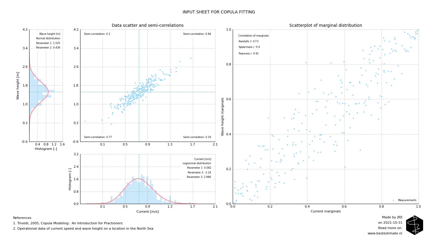
Below image shows the two variables measured at the same time and their respective probability density functions. It is obvious that wave and currents are heavily correlated, but their distributions are not normal. This poses difficulties for simulation of different plausible scenarios. How do you sample from two (already complex) distribution functions. A Copulas is an outcome for this since it can model the joint variability for two distributions, whatever they are.
A semi-correlation analysis (correlation coefficient of data in each quadrant) always needs to be performed (see Figure below). It can be observed that the correlation in the top right quadrant (where the extreme values are) is highest. If correlation between quadrants differs copulas are even required to describe joint variability properly. To fit a copula the data is transformed to the marginal domain, so to values between 0 and 1. After this is done the correlation is computed for those data points (between 0 and 1). That is the trick. This all is required to objectify the analysis (independent of the probability density function). In other words...

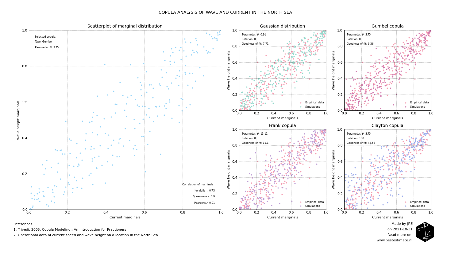
With the API four potential copulas are fitted to the marginally distributed data. These copulas are named Gaussian, Clayton, Gumbel and Frank. All four show a typically different tail behavior. Where the Gaussian is most famous the other three are more suitable to model non-symmetric correlations (as in our example). Based on the goodness of fit tests performed in the API it appears that the Gumbel copula fits best. This is logical since the Gumbel copula fits also has a heavy correlated upper right tail.

API UPDATE #1 - COPULA ASSESSMENT
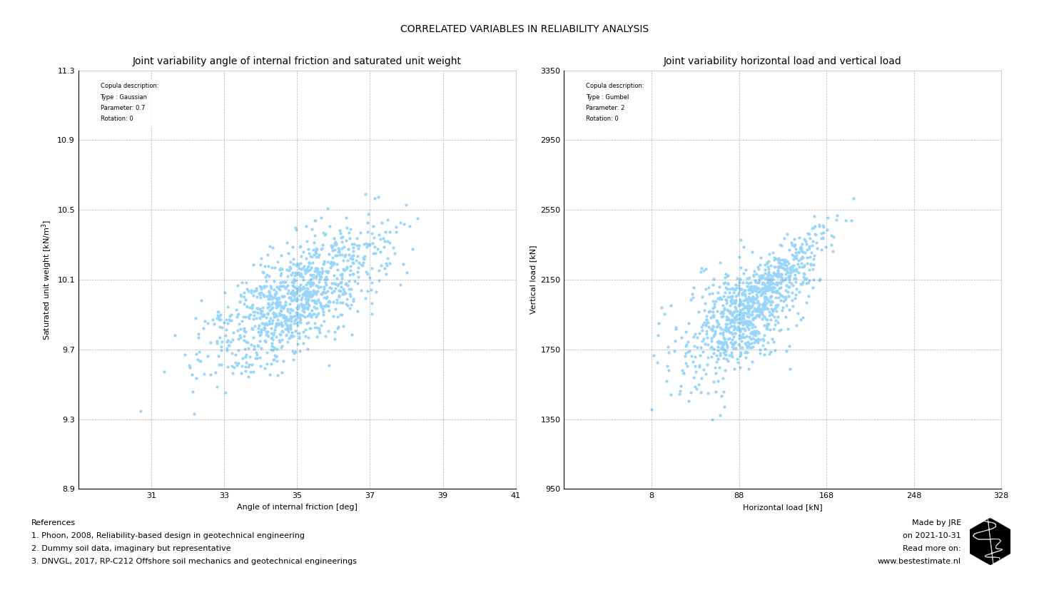
The copula analysis is added to the API and can be found on the public repository. Please note that after you performed the analysis and selected the copula you can also use it directly in reliability analyses. In the previous newsletter it was shown that joint variability can have a large effect on the safety of your analysis. Below figure shows the samples in a Monte Carlo analysis originating from a given copula and probability density functions for multiple input parameters. Try it yourself with this example.

Note that depending on the variable input the copula can also be rotated or or used with a self-selected parameter. All is explained on the public repository. Copulas are quite complicated and should be used in the right way, please reach out if you would like to know more or read it in on their background yourself. Bad usage of Copulas caused the financial crisis, so it is a popular topic on the internet.
FOOTNOTE
Please note that I run this service besides my job at Temporary Works Design. It is my ambition to continuously improve this project and publish corresponding newsletters on new innovations. In busy times this might be less, in quiet times this might be more. Any ideas? Let me know!
