JANUARY 2023 - EXTREME VALUE DISTRIBUTION
Designs and operations are often tailor made for extreme conditions as these determine the required strength. Extremes are often determined subjectively or based on previous measurements. This blog explains how to apply generalized extreme value distributions on a typical design problem. Return periods for different parameters can be estimated after post-processing the data and fitting the distributions.
TOPIC OF TODAY - #1 (GENERALIZED) EXTREME VALUE DISTRIBUTION
The mechanical properties of various materials may be affected by temperature fluctuations. This is particularly the case for polymers at low temperatures. Therefore, it is crucial to determine the minimum anticipated temperature throughout the lifespan of a project. In the case of civil and offshore structures, the design lifetime can extend up to 100 years.
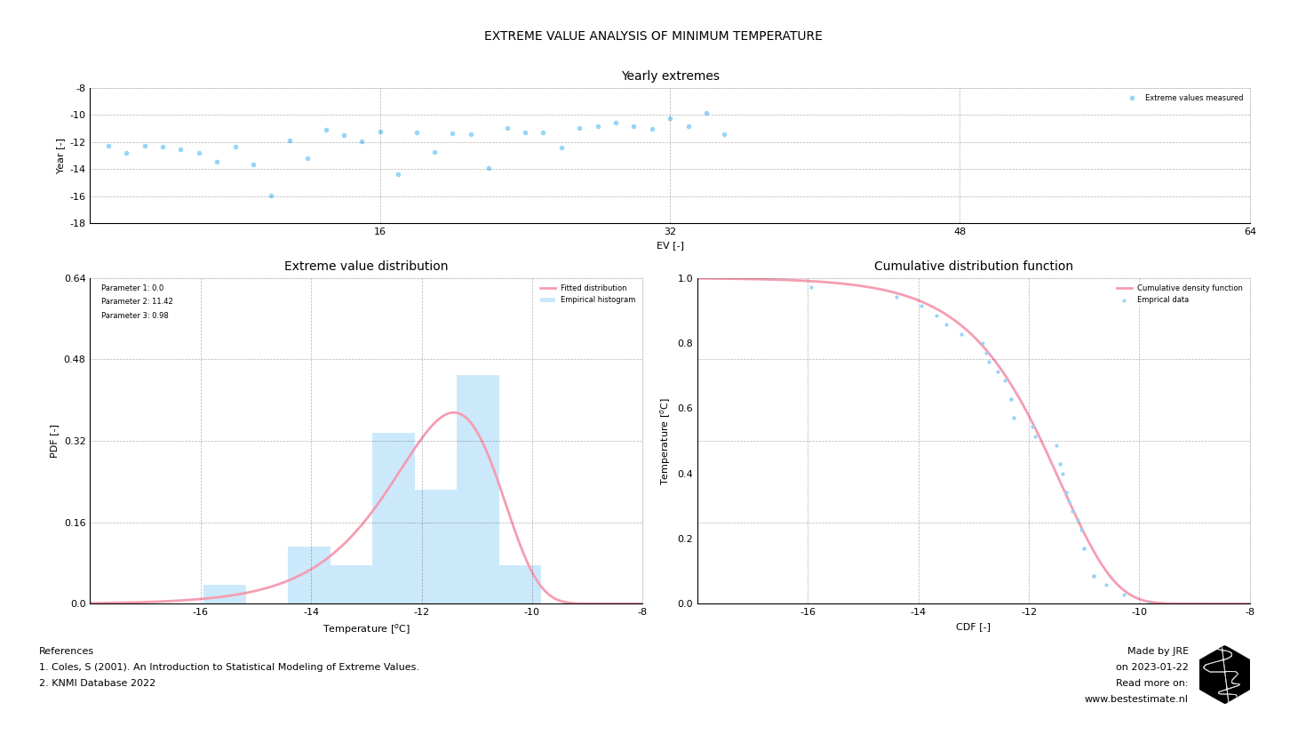
In order to determine the extreme values over the lifespan of a structure, data collection is necessary. In the North Sea, there are several stations that measure temperature. In this case, a dataset containing over 35 years of measured data is used for the study of extremes. The yearly extremes are extracted and depicted at the top of the figure below. Subsequently, a Generalized Extreme Value (GEV) distribution is fitted. In short: a GEV is a distribution that describes the probability of a yearly extreme (for this sampling interval). The fitting process is identical to that of probability density functions describing instantaneous parameter values. Refer to a previous blog for further explanation. As depicted in the figure, it is much more likely for a yearly minimum of -12 degrees to occur than a temperature of, for example, -15 degrees.

TOPIC OF TODAY - #2 RETURN PERIODS
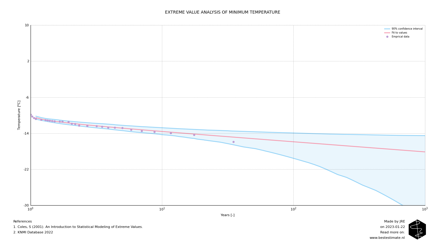
While the distribution of extremes in the figure above provides valuable information, it can still be challenging to select a minimum temperature. Computing the temperature for different return periods can assist in this. As we are computing yearly maxima, the cumulative distribution function calculates the likelihood of exceedance in years. As depicted below, a temperature of -15 degrees is expected every 100 years according to the computed GEV. This also indicates that, based on the current selected distribution, the lowest value ever measured (about -16 degrees) appears to be an outlier.

However, this analysis is based on only 35 measurements, which may not be sufficent to draw accurate conclusions for the coming 100 years. A bootstrap analysis on the extremes can help to compute lower and upper bounds which are expected. The procedure is straightforward; 1000 bootstraps are created based on the measured yearly maxima, and a GEV is fitted to all the bootstrap samples. Based on these fitted GEVs, a 90% confidence interval is established. As depicted, the 100-year return period values ranges between -14 and -18 degrees. The latter value is the most suitable for use as a design value, which is almost 3 degrees lower than the lowest temperature ever measured. It is therefore unconservative to just take the minimum measured value of -15 degrees. The extreme value distribution helped reducing the risks over the lifetime of the structure you are designing.
FOOTNOTE
Please note that I run this service besides my job at TWD. It is my ambition to continuously improve this project and publish corresponding blogs on new innovations. In busy times this might be less, in quiet times this might be more. Any ideas? Let me know!
