BOOTSTRAPPING & DISTRIBUTION FITTING
- How sure am I that I have measured enough outliers?
- What is a proper parameter estimate for further use in my work?
- What is the likelihood that I will encounter the worst case situation in field?
- How can I describe the variability of my parameter correctly?
Disclaimer. Privacy. Unsubscribe. Reach out.
bootstrap analysis
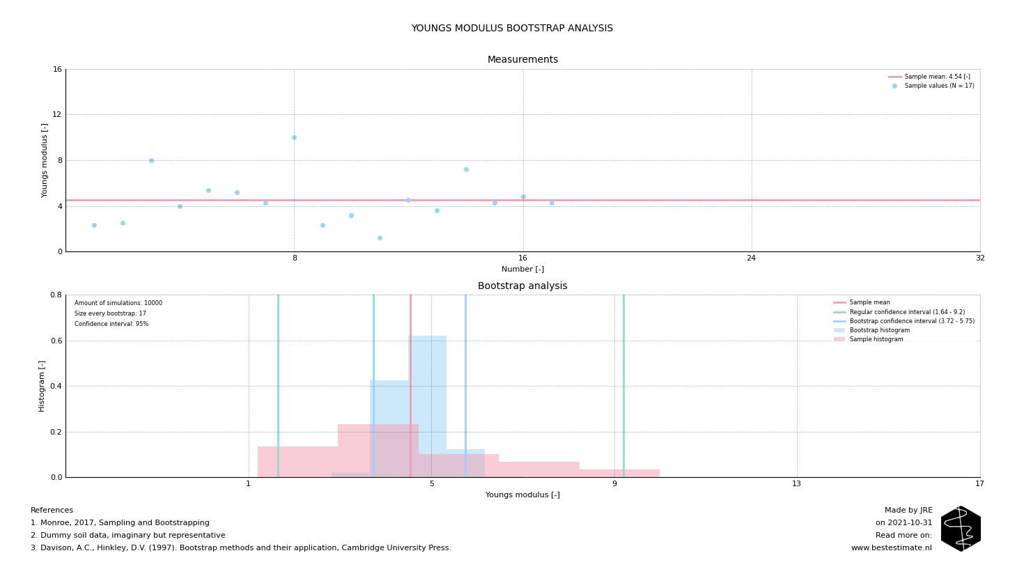
Bootstrap analyses show insights in how accurate you can estimate the mean value of a parameter of interest. Often measurements are expensive and cannot be performed unlimited. Figure 1 shows an example of 17 measurements of the Youngs Modulus (stiffness) of a soil type. This is an important parameter to estimate deformations of (for example) a temporary placed foundation. Bootstrapping is a technique which is used to estimate the variability possible in the mean value. It uses random sampling with replacement. Since a mean value is often used to get insights in deformations it is important to know whether we can actually estimate it based on the 17 measurements available.

Figure 1, Bootstrap analysis performed on Youngs Modulii estimated during a site investigation campaign
Table 1 shows the actual best estimate of the mean can vary up to 40-50%. As visible variation in settlement between 76 mm and 148 mm is likely to be expected. Conventional estimates based on the mean might lead to unsafe design since limited data is available. Additionally any safety factor which is applied is always arbitrary and only provides perceived safety. A bootstrap analysis is essential for proper interpretation of calculations based on measurements.
| Description | Conventional approach | Bootstrap analysis |
|---|---|---|
| Force (F) | 4000 kN | 4000 kN |
| Foundation diameter (D) | 3 m | 3 m |
| Poisson ratio (v) | 0.25 | 0.25 |
| Youngs Modulus (E) | 4.54 MPa | 3.72 - 5.75 MPa |
| Settlement (ε) | 117 mm | 76 - 148 mm |
Table 1, Comparison between conventional analysis and a bootstrap analysis
Distribution fitting
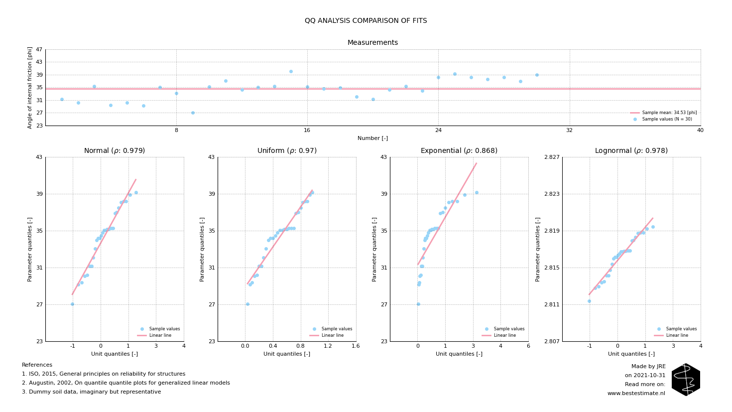
Fitting a probability density function allows everone to theoretically describe the variability of a parameter that is measured multiple times. Contrary to looking at the mean, it includes the amount and type of variation of the data. This allows for objectively estimating upper and lower bounds based on a pre-defined safety level. These analyses are often forgotten in practice and if used, performed in an over-simplified and incorrect manner. One step often misses: determining which type of distribution fits best. Figure 2 shows a Quantile-Quantile (QQ) analysis of 30 measurements of the angle of internal friction (describing the shear strength of sand). The closer the dots are to the 'unit line' the better the fit of the distribution.
Currently only 4 distribution types are supported (Uniform, Normal, Lognormal and Exponential). There are many different possibilities. These can all be implemented to make the tool more complete. Reach out if you would like an update.

Figure 2, Assessing which distribution is best suitable for further use with Quantile-Quantile (QQ) analysis
A QQ-analysis always provides an answer and is therefore of no use on checking whether sufficient data is available for a proper variability description.
After performing a QQ-analysis a 'goodness of fit' test is performed to the best fitting distribution (this is called a Kolmogorov-Smirnov test).
This test checks if the distribution is actually good enough or might be un- or overconservative.
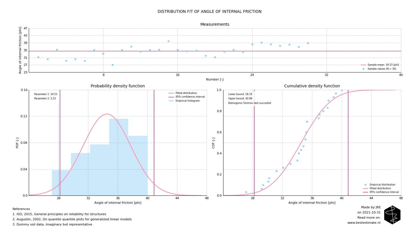
When the test result is succesfull (as stated in Figure 3) the distribution can be used to estimate upper and lower bounds of the parameter.

Figure 3, Distribution fitting of the best fitting type for the angle of internal friction
A conventional method to determine ultimate sliding capacity of a foundation would use lower bound estimate of 29 degrees and a safety factor of 1.2.
On the other hand, a probabilistic approach uses an objective (in this case 95%) confidence interval.
This gives considerably more information.
Table 2 shows the lower, mean and upper bound horizontal load which can be applied based on the quantified variability of the angle of internal friction.
As visible the allowed horizontal load can safely be increased by 20% which results in feasibility for application in tougher conditions.
| Description | Conventional approach | Lower bound | Best estimate | Upper bound |
|---|---|---|---|---|
| Vertical load (V) | 4000 kN | 4000 kN | 4000 kN | 4000 kN |
| Angle of internal friction (φ) | 29.0 deg (24.8 factored) | 28.2 deg | 34.5 deg | 40.9 deg |
| Allowed horizontal load (H) | 1848 kN | 2144 kN | 2751 kN | 3460 kN |
Table 2, Comparison of conventional approach to a detailed study using distribution fitting
Truncated distributions
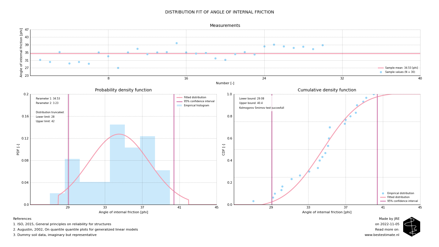
The analysis above is already a major improvement if you would compare it to current practice. Nonetheless, further improvements are possible. For example by limiting the fitted distributions to physically possible and expected parameter values. This is possible by means of truncation. In this process the tails of the distribution can be removed. This avoids sampling from domains in the parameter space which are physically infeasible (in this case for example a value of 25 degrees). Figure 4 shows a truncated distribution.

Figure 4, Truncated distribution fit using only expected values of the angle of internal friction for the specific soil unit
References
- Monroe, 2017, Sampling and Bootstrapping
- Verruijt, 2012, Soil mechanics
- Augustin, 2002, On quantile quantile plots for generalized linear models
- ISO, 2015, General principles on reliability for structures
- Stephens, 1974, EDF statistics for goodness of fit and some comparisons
