JULY 2023 - FORECASTING
Often statistics are all about understanding datasets. But it would be most desirable if we could forecast the future based on the past. This is not easy, but can provide a lot of value if performed correctly. This blog elaborates on a practical case study on predictive maintenance by means of greasing.
TOPIC OF TODAY #1 - FORECASTING
A lot of statistics in the offshore industry focus on determining conservative values. In most design cases related to safety, this is more than enough. However, in some cases, you also would like to know what is coming. Examples are the prediction of wear, fuel consumption, cycle times, and time until maintenance. Data often has significant fluctuation. Therefore, a fixed value or linear estimate cannot provide the reliability required. Good use can be made of prediction algorithms like ARIMA. ARIMA is a get-together of three different parts:
- AutoRegressive (AR): This basically says that past measurements are used to predict future values avoiding direct use of the single value before.
- Integrated (I): This basically means that we do not think from the perspective of values but from the differences between individual measurements.
- Moving Average (MA): The moving average part of the algorithm eliminates the influence of short term fluctuations thus making it more robust.
TOPIC OF TODAY #2 - ARIMA ANALYSIS
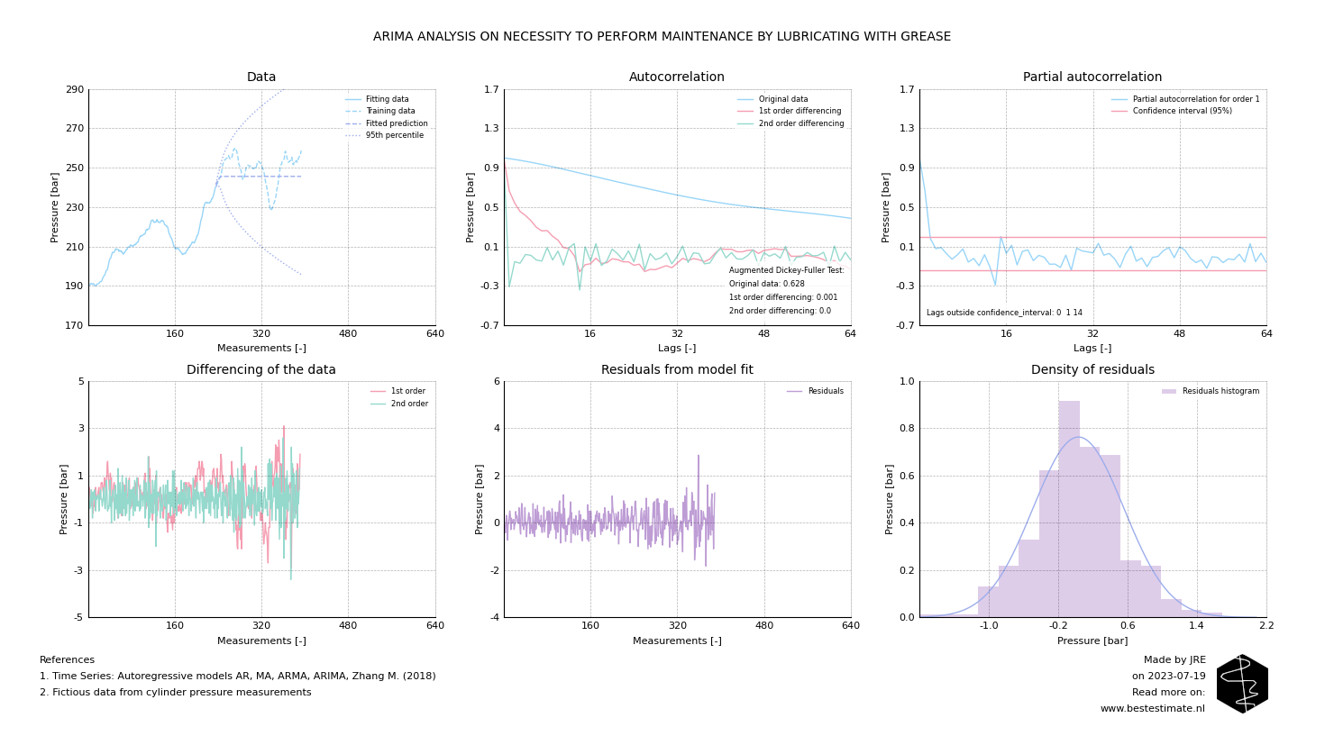
In this blog, ARIMA is applied to a case study where a skidding system with a hydraulic cylinder requires grease once in a while. Greasing too much is time-consuming, costly, and bad for the environment. Greasing too little can cause failure during operation or excessive wear. In this case, the maximum cylinder pressure at which greasing should really start is 300 bar. The figure below shows how we determine the input for an ARIMA analysis:
- The first plot (top left) shows a split of the existing data in fitting data (first half) and training data (second half). We do this to check if our model fits the data properly before we apply it in practice. Lots of more fancy stuff can be done, but in this case we will keep it simple.
- The second plot (top middle) shows the autocorrelation plot for multiple orders of differencing (shown in the bottom left). In short we want a low autocorrelation assuring us that the differences do not have hidden trends.
- The third plot (top right) shows the partial autocorrelation for the selected degree of differencing (in this case 1). This shows if there is a returning trend at different lags in the data (like for example a spike at every 10th measurement).

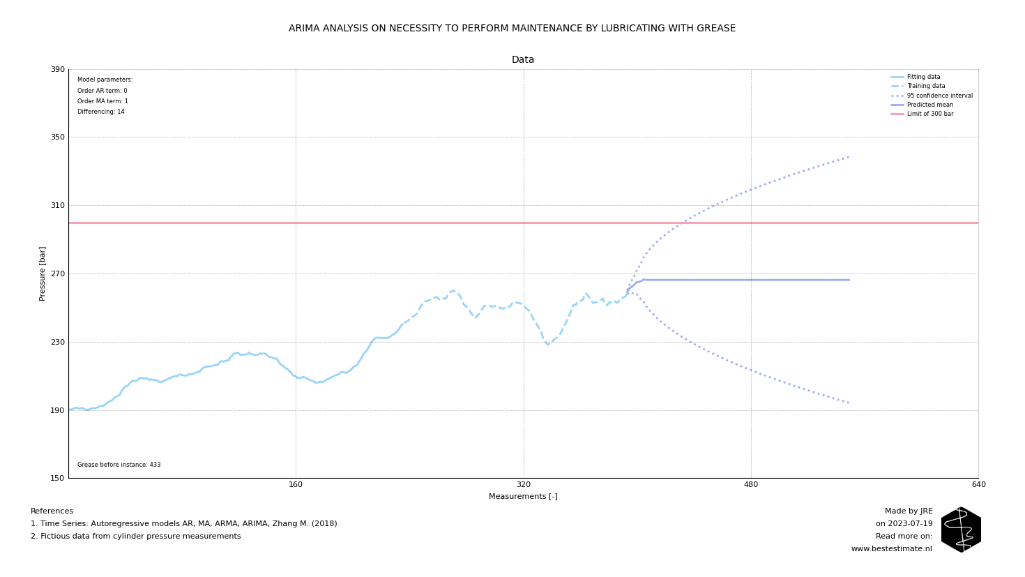
Good, the model is fitted! Now we can start forecasting. Well, that is very simple, and the outcome is visible in the figure below. If you would plot a straight line through our measurement data, the expected maintenance date would be on day 600. However, our ARIMA analysis (which takes into account past fluctuations and underlying patterns) shows that it could also be within 433 days. So if you have mission-critical equipment depending on proper lubrication, it is wise to plan maintenance within 433 days.

FOOTNOTE
Please note that I run this service besides my job at TWD. It is my ambition to continuously improve this project and publish corresponding blogs on new innovations. In busy times this might be less, in quiet times this might be more. Any ideas? Let me know!
